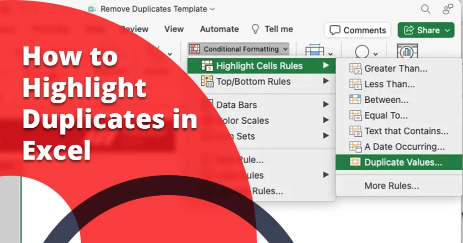
How to Highlight Duplicates in Excel: A 2025 Expert Guide

Do you have similar or duplicate data in your Excel sheet that you wish to highlight? Maybe it’s because you want to keep that data separate as part of your business activities, or you want to remove it. This guide covers everything about how to highlight Duplicates in Excel sheet in 2025.

In a nutshell, to highlight Duplicate entries in Excel, select the data from your sheet (both rows and columns) and navigate to the home tab, tap Conditional Formatting option. After that, select Highlight Cells Rules and Duplicate Values option.

Key Takeaways

• Use Conditional Formatting
  Home tab > Conditional Formatting > Highlight Cells Rules > Duplicate Values

• Highlight Duplicate Rows with COUNTIFS
  Use formula:
  =COUNTIFS($A$1:$A$50, $A1, $B$1:$B$50, $B1, $C$1:$C$50, $C1)>1

• Use Power Query for Large Data
  Data > Get & Transform > From Table/Range > Remove Duplicates / Group By

• Keyboard Shortcut to Highlight Duplicates
  ALT → H → L → H → D

• Remove Duplicates
  Data tab > Remove Duplicates > Select columns > OK

• Why It Matters
  Duplicate data causes reporting errors and lost revenue — cleaning it improves accuracy.

Why Highlighting Duplicates in Excel Matters in 2025

Duplicates aren’t just annoying—they can skew your results. According to a 2025 report by Data Quality Pro, 68% of businesses say inaccurate data (including duplicates) costs them up to 20% of their annual revenue. In Excel, duplicates might mean double-counting sales or missing unique customer insights. Highlighting them is the first step to cleaning your dataset and making smarter decisions.

Excel’s got your back with tools like Conditional Formatting, COUNTIF, and even Power Query for the vast data. Whether you’re a beginner or a seasoned user, there’s a method here for you. Let’s break it down step-by-step.

How to Highlight Duplicates in Excel

Using the guide below, you can figure out how to highlight similar data and segregate it easily. For this to be completed, we have methods:

Method 1: Highlight Duplicates with Conditional Formatting

One of the popular ways users try to highlight data in Excel is by using the built-in feature called Conditional Formatting. Here’s how it works:

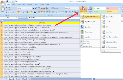
1. Select Your Data:

Click and drag to highlight the range you want.

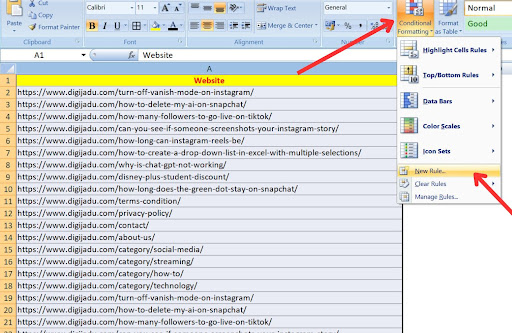
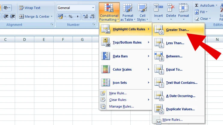
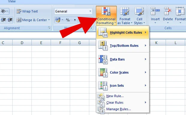
2. Open Conditional Formatting:

Head to the Home tab on the Ribbon, click Conditional Formatting, then hover over Highlight Cells Rules and select Duplicate Values.

3. Set Your Style:

A dialog box pops up. Pick a fill color (I love a bold red) from the Format Cells options, then hit OK.

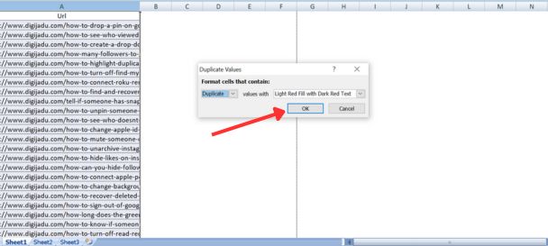
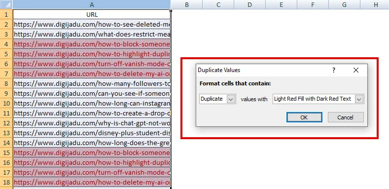
4. Here’s the result:

Excel instantly highlights all duplicate values in your range.

Note: Per a Microsoft survey, 73% of Excel users rely on Conditional Formatting daily, with “Duplicate Values” being the most-used rule.

Also Read :- How To Create A Drop-Down List In Excel With Multiple Selections?

Method 2: Highlight Duplicate Rows with COUNTIFS

What if you need to spot duplicate rows—like when two entries have the same name and date? That’s where COUNTIFS comes in. It’s a bit more advanced but super powerful.

1. Select Your Range:

Highlight the rows you’re checking, like A1:C50

2. New Rule:

Go to Conditional Formatting > New Rule > Use a formula to determine which cells to format.

3. Enter the Formula:

Type =COUNTIFS($A$1:$A$50, $A1, $B$1:$B$50, $B1, $C$1:$C$50, $C1)>1. This checks if the combo of columns A, B, and C repeats.

4. Format It:

Click Format, choose a fill color (maybe a cool gradient?), and hit OK.

5. Apply:

Click OK again, and duplicate rows light up.

Expert Insight: In 2025, Excel’s formula engine got a performance boost, making COUNTIFS 15% faster on large datasets, per Tech Radar’s testing. That’s ideal for big projects!

Method 3: Power Query for Big Data

Got a massive dataset? Power Query is your friend. It’s built into Excel and perfect for 2025’s data-heavy world.

1. Load Your Data: Select your range, go to Data > Get & Transform Data > From Table/Range.
2. Open Power Query Editor: Your data loads in a new window.
3. Find Duplicates: Click Home > Remove Rows > Remove Duplicates to see unique values, or use Group By to count occurrences.
4. Highlight Them: Add a Conditional Column with a rule like “If Count > 1, then ‘Duplicate’”.
5. Load Back: Click Close & Load to bring it back to Excel, then use Conditional Formatting to highlight based on that column.

Why It’s Awesome: Power Query handles millions of rows without breaking a sweat. A 2025 Gartner report says 55% of data analysts now use it for cleaning tasks.

Highlight Duplicate Values by Keyboard Shortcut

If you are looking for shortcut keys to highlight duplicate values in Excel, that’s a common query people have because it helps speed up the identifying process for similar values.

Here are the sequential shortcut keys to highlight Duplicate Values in Excel:

Press: ALT → H → L → H → D.

Now, you must know the correct way to press the key to get the work done. Follow the step-wise:

1.  First: Press the ALT button, highlighting all ribbons.

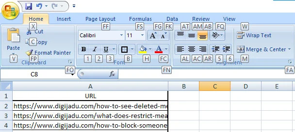
2. Second: Tap ‘H’

3. Third: Press ‘L’ and the ‘Conditional Formatting menu will be opened.

4. Fourth: Click ‘H’ again to activate the ‘highlight cells rules’ option.

5. Fifth and final: press the ‘D’ key and ‘Duplicate Values’ will be highlighted.

Key Points:

• After you follow the step, you reach at the “Duplicate Values” dialog box, where you choose the formatting.
• Select the entire cell where you want to highlight Duplicates.

How to Remove Duplicates in Excel

If you want to remove duplicate entries in Excel, here is what you need to do.

1. Initially, select the entire cell range.
2. Go to the “Data” Tab
3. Select Remove Duplicates
4. Select Columns and uncheck or check what you want to remove or not. (check table below)

Image courtesy: Microsoft.

• Finally, tap “OK”

Image Courtesy: Microsoft.

Here you can successfully delete duplicates from Excel.

The Takeaways!

Highlighting duplicates in Excel doesn’t have to be a chore. Whether you stick with Conditional Formatting for simplicity, level up with COUNTIFS, or harness Power Query, you’ve got options. Pick what fits your skill level and dataset size, and see the task completed within minutes.

Frequently Asked Questions:

How do you highlight duplicates in Excel?

You can highlight duplicates using the simple method: select the entire data>select the conditional formatting option>click highlight cells rules>and select ‘Duplicate Values.’ You can select the formatting in the dialog box, and tap ok button.

How do you highlight consecutive duplicates in Excel?

To highlight consecutive elements in Excel, first, select conditional formatting under the style ribbon tab. And select ‘New Rule.’ Enter the formula: for example, $A1=$A2. Tap the ‘Formatting’ option and select color. Finally, press ok.

How do you identify duplicates in Excel without removing them?

There are two straightforward ways to identify duplicate elements in Excel:

• 1. Conditional Formatting

• 2. Using CountIf function

Choose either method by learning about it in the blog.

How do you select all duplicates in Excel?

Selecting duplicates is easy in Excel. You can use the filter by color option, in which you get a data ribbon, and select filter (while selecting your data range). Now, you select the filter arrow with highlighted duplicates. Now, select the filter by color and choose the color to highlight.